Appendix E
Q-Day Model
Bottom-Up vs. Top-Down Predictive Models
BOTTOM-UP
Resource Estimates
- More accurate and rigorous
- Architecture-specific
- Hard to compare across approaches
- Forecasts requirements, not trends
TOP-DOWN
Predictive Models
- General enough for multiple approaches
- Produces an explicit timeline forecast
- Additional assumptions reduce scientific precision
"All models are wrong, some are useful"
Q-Day Model Framework
Three Constraints Define Q-Day
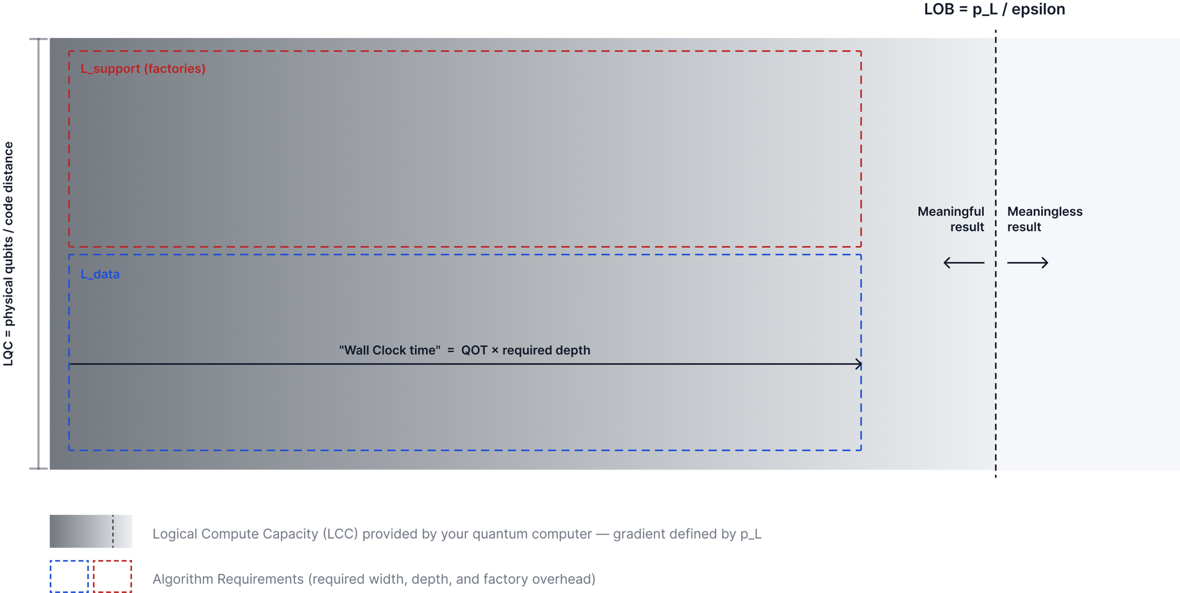
LQC ≥ Circuit Width
The number of logical qubits available must be at least as wide so as to accommodate the maximum number of logical operations at any step in the computation.
LOB ≥ Circuit Depth
The number of logical operations available (above the failure threshold epsilon) must be at least as wide as the number of required parallel logical operations at the highest point.
QOT × LOB ≤ 100 days
The total "wall clock time" (QOT × LOB) must be on a timescale that could be considered "cryptographically relevant." In this model, we define that scale as <100 days.
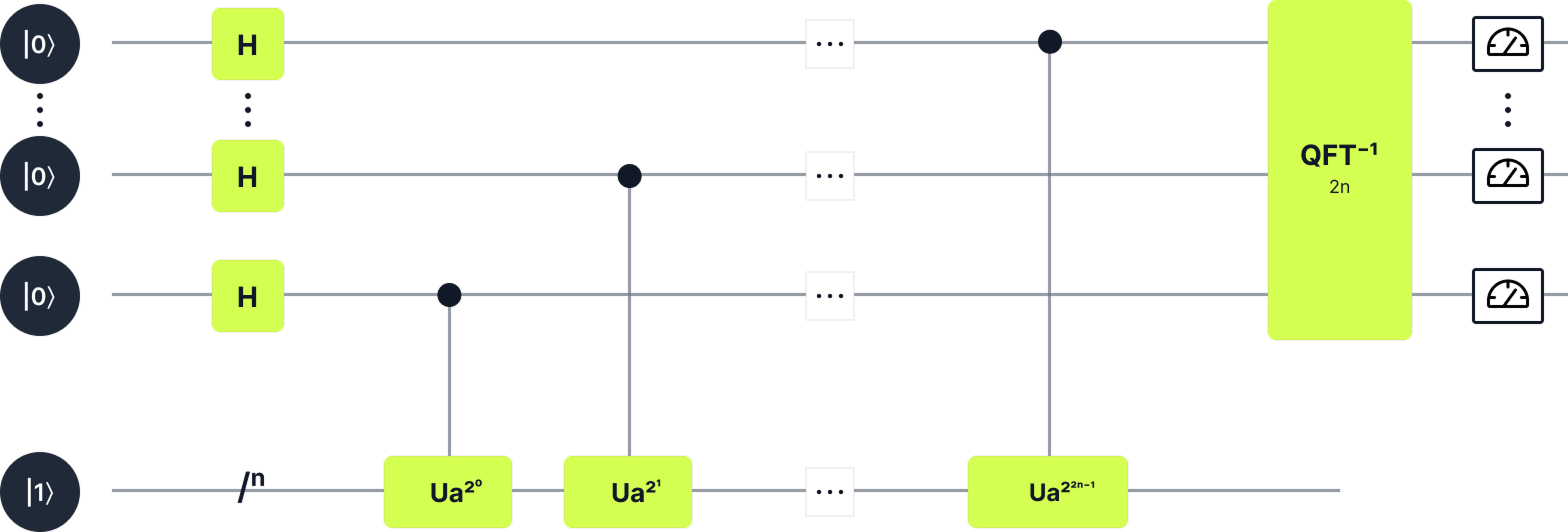
A Simplified Model for Shor’s Algorithm
Reality
Quantum Phase Estimation
Shor's Algorithm Subroutine
4 Steps to Fault-Tolerant Quantum Computing
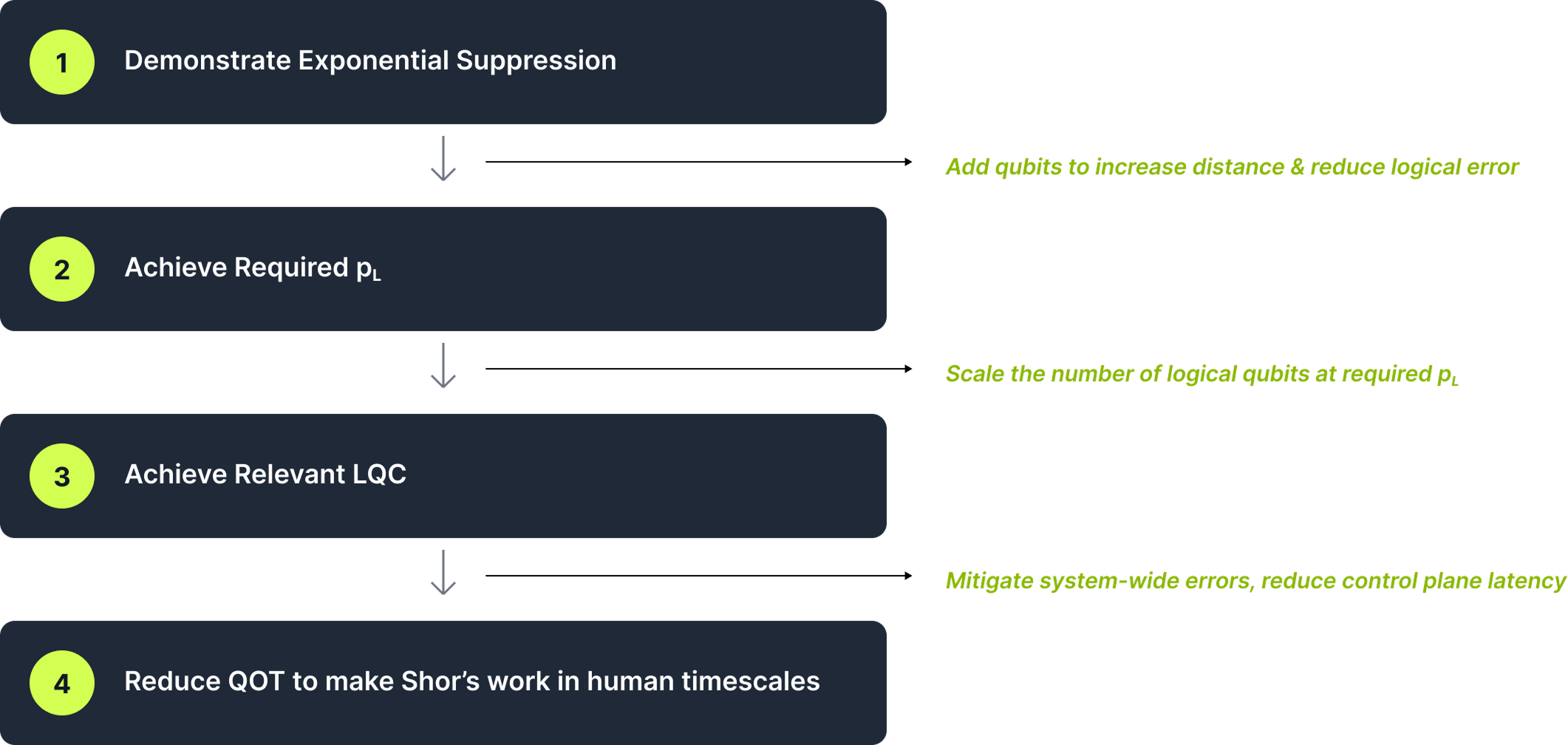
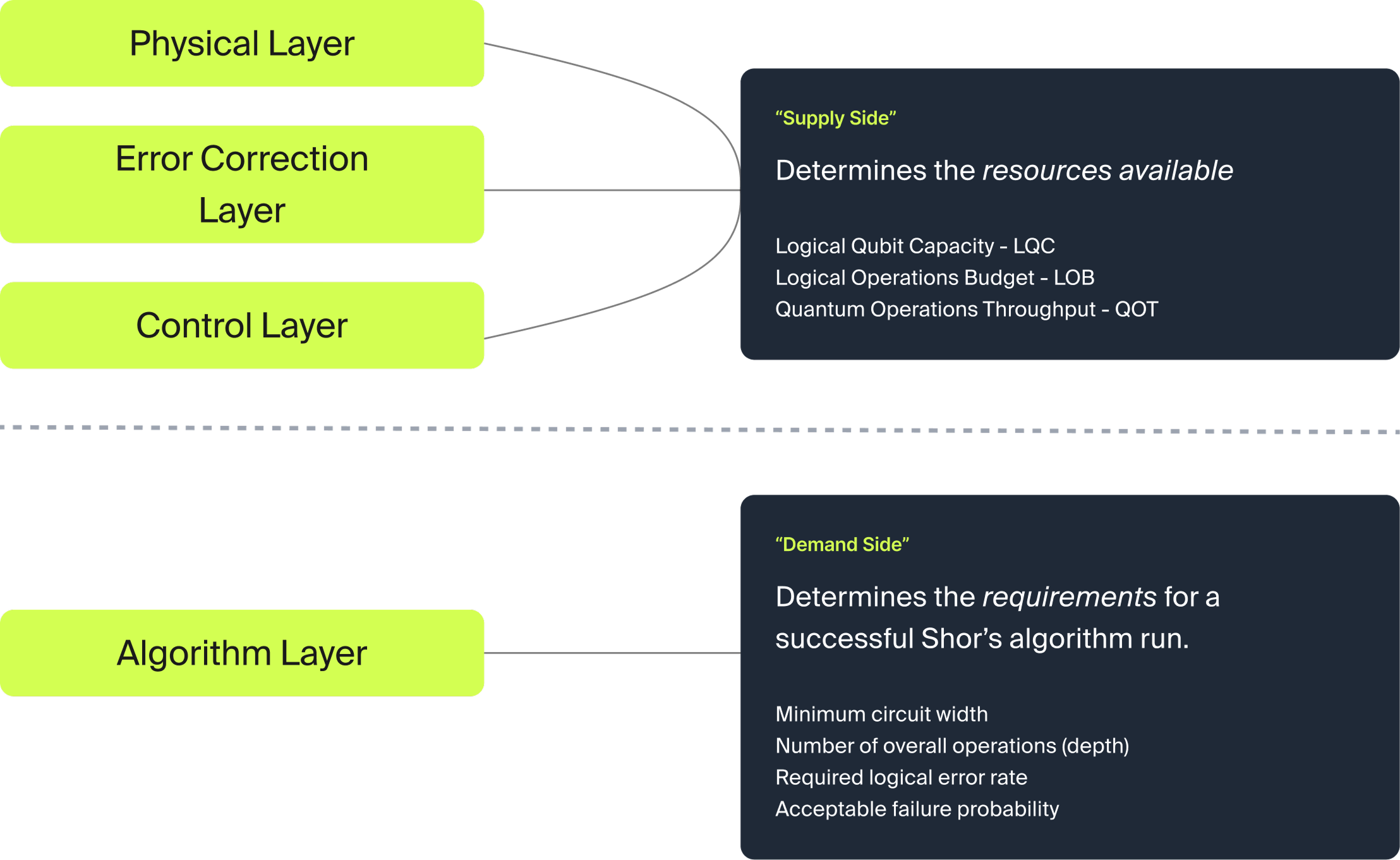
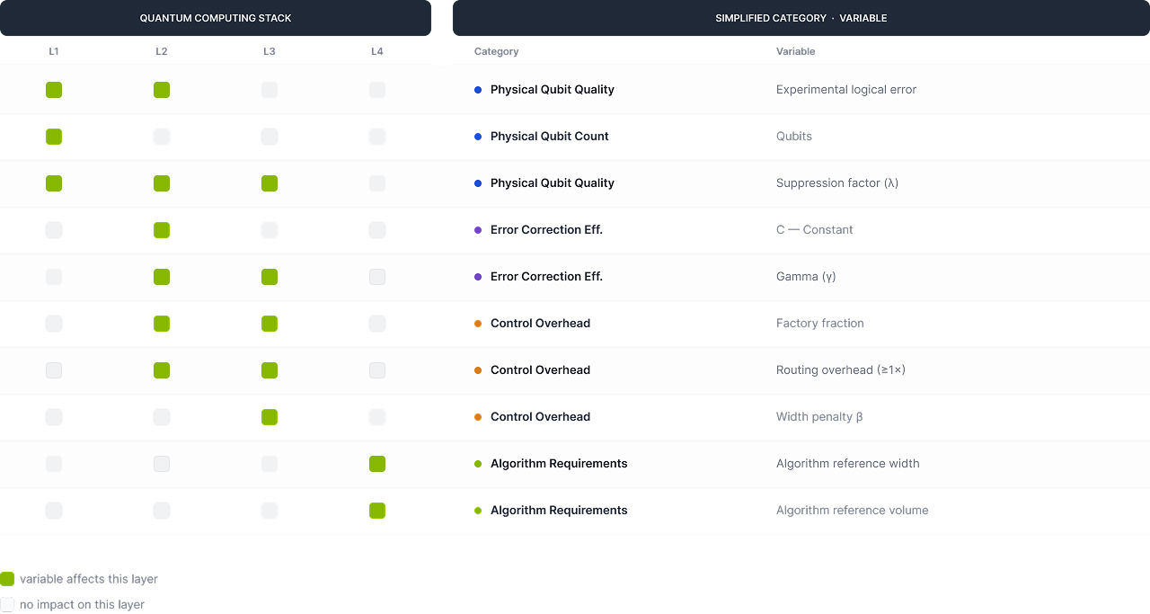
Variable Definitions — Quantum Resources “Supply”
- Experimental distance
- the code distance used as a baseline.
- Experimental logical error (pL)
- the logical error rate achieved at that distance
- Qubits
- the number of physical qubits available
- Suppression Factor
- the impact of increasing distance on the logical error rate at each step
- C — constant
- the constant factor penalty applied associated with with a given code
- Gamma (γ)
- the exponent "overhead" for the code. E.g. for surface code patches, γ is 2
- Cycle Time
- time required to complete one quantum error cycle (QOT)
Variable Definitions — Algorithm Overhead “Demand”
- Failure Tolerance
- the failure rate per run of a quantum algorithm
- Factory Fraction
- % of logical qubits dedicated to magic state production
- Target Logical Error/Cycle
- logical error rate
- Routing Overhead
- penalty applied to LQC to account for qubit routing reqs
- Algorithm Reference Width
- Minimum required width given by the algorithm
- Algorithm Reference Volume
- The total number of required operations for the given Shor's variant being targeted
- Width Penalty
- "effective" additional width required over the algorithm reference width to account for a variety of other failures/errors
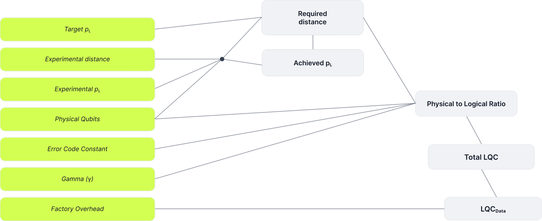
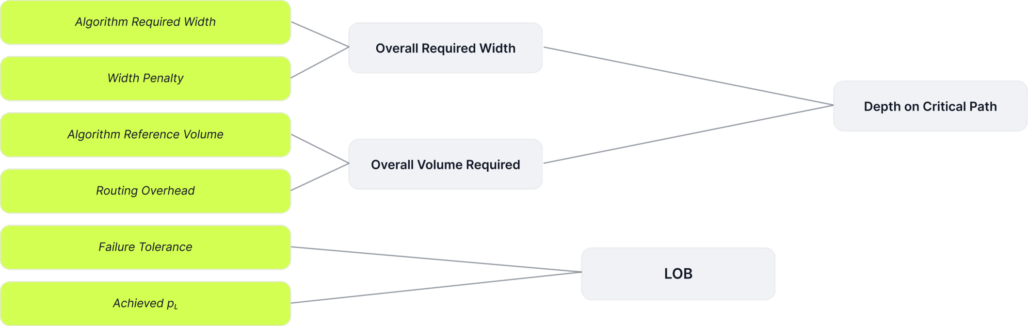
Variable Relationships
Model Mechanics — Supply Side
Model Mechanics — Demand Side
Notable Assumptions
Error Correction Anchored to Surface Codes
The physical-logical qubit overhead and error correction calculations are effectively anchored to surface codes for ease of modeling. Improvements stemming from more efficient codes like qLDPC codes are captured effectively by reducing the gamma (γ) parameter in the exponent
Cycle Time Fixed at 10 µs
Cycle time is 10 microseconds, roughly equivalent to superconducting qubits today. This is held as a constant; different scenarios could be considered with slower cycle times more in-line with modalities like neutral atom/trapped ions
Algorithm Target is RSA-2048 via Shor's
The algorithmic resources are based on RSA-2048. It's entirely possible (in fact, likely) that elliptic curves require less width/depth, because Shor's scales logarithmically based on key-length, and ECC keys are 256 bits (vs 2048 bits).
Variable Ranges
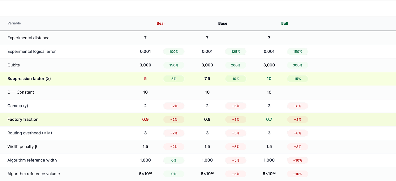
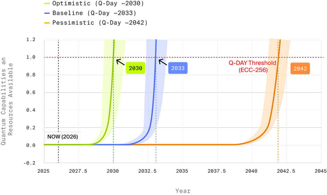
Model Output
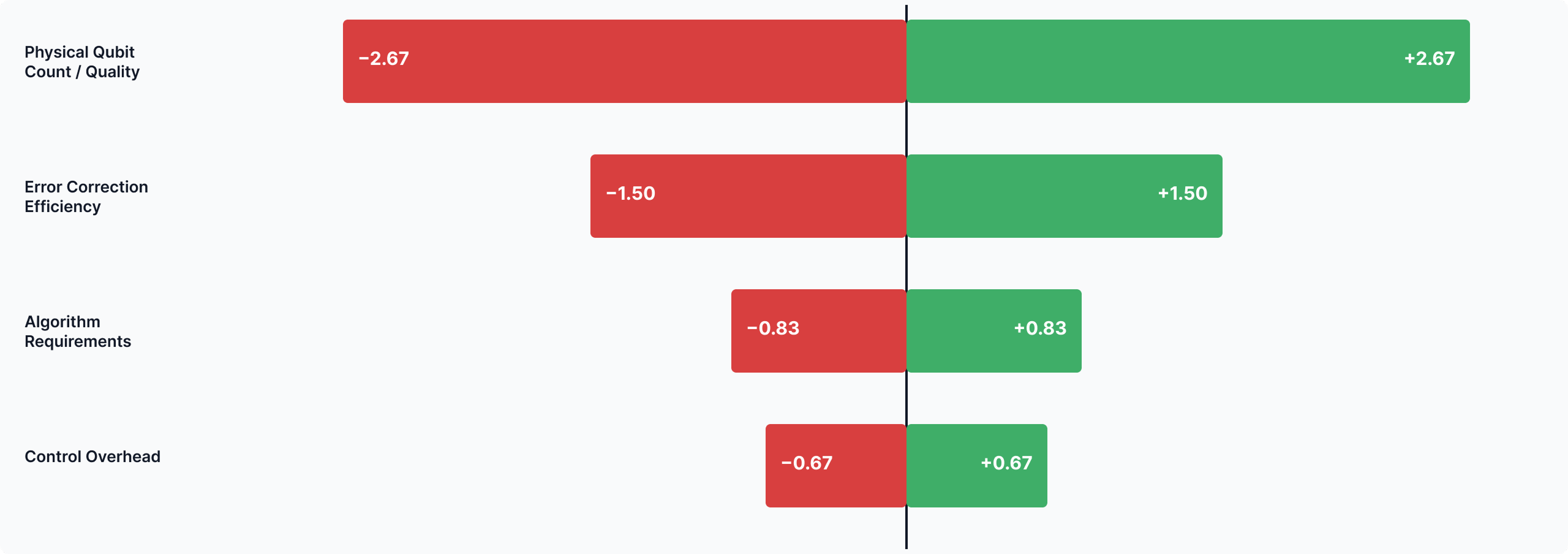
Sensitivity Analysis — Variable Impact on Q-Day
Model Idiosyncrasies
WHERE THE MODEL DEPARTS FROM PHYSICS
The point where the model probably breaks down from physics most clearly is the error suppression factor, α
The reason for that is that, in effect the model works “backwards” from what you would do in real life, which is define a distance and then calculate the logical error rate based on that. Instead, here we “hard code” the logical error rate based on the algorithm requirement (we hold it at 10⁻¹⁵), and then calculate the distance based on that.
This massively inflates code distance relative to published resource estimates, so we crank up the suppression factor to compensate. Suppression factor is typically around 2 for recent Google, Quantinuum experiments. Our model assumes a range of 5–10 to start. Optimistic suppression factor estimates range to 25.
Key Takeaway — LQC is the Dominant Constraint
KEY TAKEAWAY 1 OF 3
Logical Qubit Capacity ≥ circuit width is the dominant constraint, assuming the threshold theorem holds and correlated errors do not dominate at scale
This is consistent with Gidney’s 2025 resource estimate, and the Google Willow demonstration: once you have below-threshold error correction, you can effectively “buy” LOB by adding more physical qubits (increasing the distance of the code to lower the logical error rate).
The farther below threshold, the greater “headroom” for correlated errors at scale. So the physical error rate (defined by the physical qubit) and the threshold (defined by the error correction regime) still matter.
Key Takeaway — Reliability and Code Overhead
KEY TAKEAWAY 2 OF 3
Once below threshold, reliability becomes easier to scale, while code overhead becomes the main factor limiting LQC.
Surface codes are well studied, but they require a number of physical qubits that scale quadratically with distance. Newer qLDPC codes reduce that overhead making each physical qubit added count for more.
Better codes drive down the number of physical qubits needed to produce & connect, a clear example of a positive feedback loop.
Key Takeaway — Algorithm Design and Q-Day
KEY TAKEAWAY 3 OF 3
The algorithm design sets the "bar" for cryptographic relevance, and optimizations there potentially have a major impact on Q-Day timelines
Note that algorithm design is not independent from architecture design. In fact, this is a hardware/software co-design problem.
The fact that LQC is the bottleneck according to this model is largely a result of the algorithm. However, time–space tradeoffs are not “free”; below a certain width, the LOB tends to grow quickly.
Key Model Takeaways
POSTSCRIPT — DECADE BEYOND Q-DAY
Barring extremely fast cycle times, or massive algorithm optimizations, short-range attacks are going to be unfeasible for at least a decade beyond Q-Day
Cryptographic Relevance is Subjective
Cryptographic relevance is subjective, but the reality of the resource requirements for Shor's algorithm provide a lower bound required volume.
Even at Best-Case Hardware Speeds…
Even at superconducting-qubit speeds and LQC of over 10,000 qubits, the effective time it would take to run this attack is tens of minutes
Future Work
IMPROVEMENTS UNDER CONSIDERATION
Refine input values
Refinement of input values based on new/better data & trends
Run a full Monte Carlo simulation
A full "Monte Carlo" simulation with various parameters for a more robust sensitivity analysis
Granular code-family breakdown
A more granular breakdown and separate functions based on error correcting code type (surface codes vs. qLDPC)
CODE-FAMILY TRADE-OFFS (DETAIL ON ITEM 03)
Surface codes
Surface codes have smaller constants, easier decoding, poor asymptotic scaling
qLDPC code families
qLDPC code families have larger constants, harder decoding, but much higher throughput (~k/n)
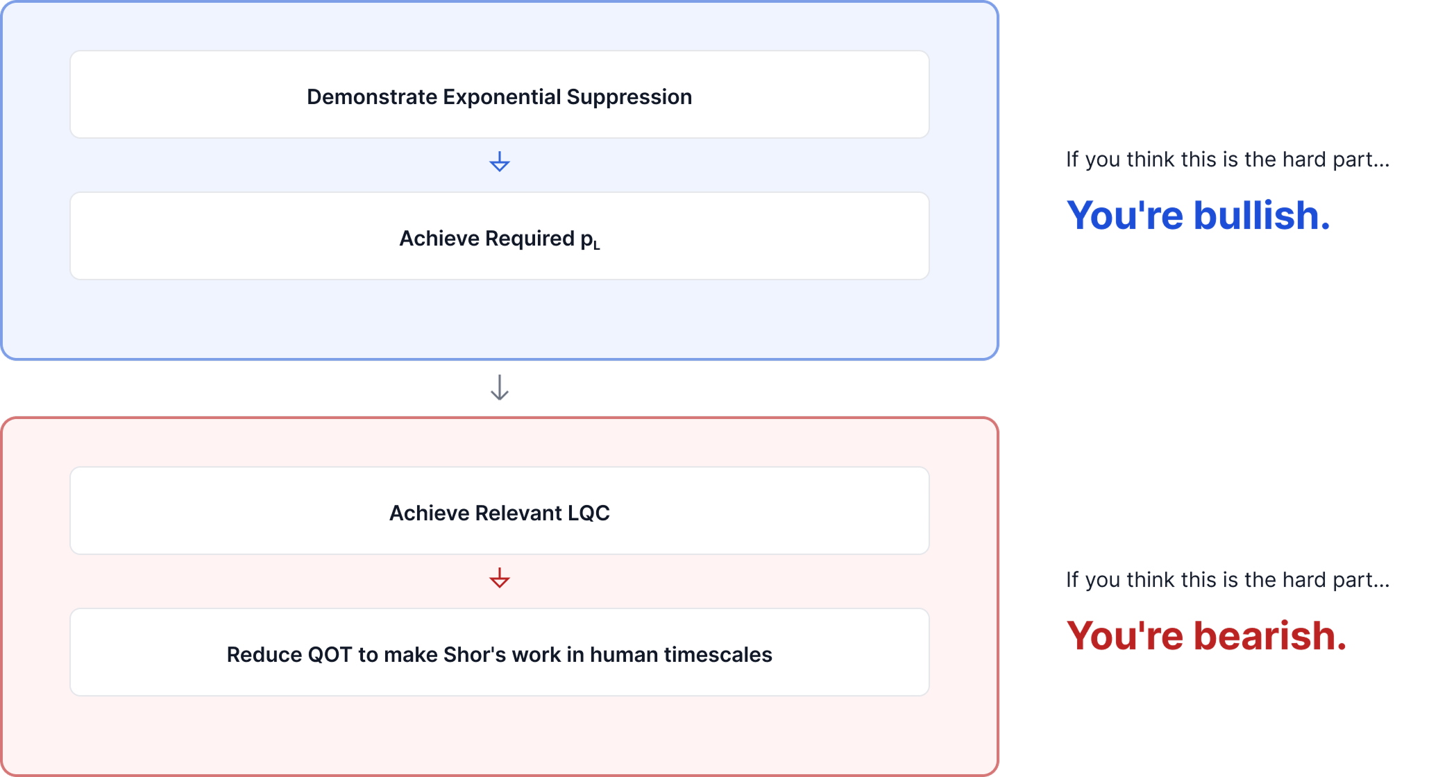
Postscript: How to Tell If You’re Bullish or Bearish Quantum