How to Build a Practical Quantum Computer

A useful way to think about large-scale quantum computation is to imagine trying to fill a giant container with water. The problem is that the container is made of a material that leaks constantly.

If you pour water into it slowly, the water simply drains away before the container ever fills. The only way to succeed is to add water faster than it leaks out.

Quantum computation has the same problem. Physical qubits constantly accumulate errors, which slowly “leak” reliability out of the computation. Error correction acts like reinforcing the walls of the container, slowing the leak. But it also makes the container inherently larger and more complicated to fill.

A quantum computer becomes useful only when the system can execute enough reliable operations before errors drain away the computation.

More concretely, we want to predict how many physical qubits operating for how long are needed to run Shor’s algorithm. But as the metaphor above illustrates, that answer depends not only on quantity, but on the quality of those qubits.

A single physical qubit is useless on its own, because it is too noisy and error-prone. It needs to be optimized for reliability in order to be useful. The threshold that we care about is the logical error rate per cycle at utility scale.

As quantum computation gets repeated over many cycles, the results get more and more unreliable. Error correction counteracts that, but adds additional computational overhead.

2025 Shor’s algorithm resource requirements [5] (Google)

~1,000,000 physical qubits and a “logical” error rate of 1 in a quadrillion per cycle are needed to break RSA-2048. Note that newer estimates focused on ECDSA are even lower.

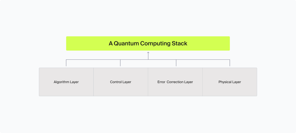
To build a CRQC is not a single engineering challenge but a stack of interdependent capabilities, where each layer depends on the one below it and feeds into the one above. Assessing how close we are to a CRQC requires a structured framework for measuring progress across the four-layer quantum computing stack [7].

A Quantum Computing Stack

Layer 1: Physics — Hardware Modalities

Everything begins with the quality of individual physical qubits. Two properties matter most: decoherence time (how long a qubit retains its quantum state before decaying) and gate fidelity (how accurately operations can be performed on it).

Because quantum mechanics governs the entire world around us, it is actually possible to realize a quantum computer in a number of different ways. These are sometimes referred to as “modalities”, which is the nomenclature we will use for the rest of this report. The choice of modality impacts the qubit quality, as well as dictates the engineering constraints for physically building the system. Higher coherence and fidelity mean fewer errors at the source, which reduces the burden on every layer above. Current state-of-the-art platforms achieve two-qubit gate fidelities between 99.9% and 99.99%. Measurement fidelity (how accurately you can read out a qubit’s state) and correlated noise (errors that affect multiple qubits simultaneously) are additional physical-layer constraints.

Modality	Key Strengths	Primary Challenges	Example Architectures
Superconducting	Fast gate speeds, mature fabrication pipelines, strong integration with classical control	Cryogenic infrastructure; wiring density; frequency crowding; correlated noise	Google Sycamore/Willow; IBM Eagle/Heron
Trapped Ions	Very high gate fidelities; long coherence times; uniform qubits	Slower gate and measurement times; scaling trap arrays; parallelization limits	Quantinuum H-series; IonQ Forte
Neutral Atoms	Reconfigurable geometry; programmable connectivity; natural compatibility with non-local codes	Measurement latency; laser stability; large-scale control complexity	QuEra Aquila; Pasqal Fresnel; Infleqtion Scorpius; Oratomic
Silicon Spin	CMOS compatibility; potential for dense integration; leverages semiconductor industry	Two-qubit fidelity; variability; crosstalk; integration complexity	Intel Tunnel Falls; Diraq Crossbar; QuTech QARPET
Photonic	Room-temperature operation; low decoherence in transit; high-speed signal propagation	Probabilistic entangling gates; large resource overhead; complex fusion schemes	PsiQuantum; Xanadu Borealis

A more detailed analysis of the different physical modalities can be found in Appendix B.

Layer 2: Quantum Error Correction

Raw physical qubits are too noisy for cryptographic computation. Error correction bundles groups of physical qubits into a single, more reliable logical qubit using specialized codes. The efficiency of this process determines the physical-to-logical qubit ratio (how much raw hardware is consumed per usable qubit), the logical error rate (how many operations can be chained before failure), and the logical cycle time (how quickly the error correction loop runs, which sets the clock speed of the overall system). In effect, it determines whether or not a given system can scale and still give a useful result.

In recent years, this aspect of the quantum computing stack has seen the greatest improvement, hallmarked by Google’s “Willow” below-threshold demonstration in 2024. The significance of this was that, by increasing code distance (using more physical qubits to encode one logical qubit), the logical error rate turns into a “dial” that can be tuned by adding more physical qubits. Before that demonstration, adding more physical qubits increased rather than decreased the logical error rate, making achieving the scale of cryptographic relevance practically impossible.

Surface Code vs qLDPC

A 200× reduction in physical qubit requirements (from 20M to ~100K) occurred in just five years, driven almost entirely by improvements in error correction efficiency — not in physical hardware. qLDPC codes require fewer physical qubits per logical qubit than traditional surface codes, dramatically lowering the bar for cryptographic relevance.

The term “logical qubit” does not imply that the error rate is zero. It means that the error rate has been reduced through error correction to a level where useful computation becomes possible. The acceptable error rate is not fixed by the hardware itself but by the algorithm being executed. Because each logical operation has a small probability of failure, errors accumulate as the circuit becomes deeper. As a result, the longer the computation (the greater the circuit depth), the lower the logical error rate per cycle must be in order for the overall computation to succeed with high probability.

Key insight: Error suppression is exponential

Moreover, because error suppression is exponential, a relatively modest jump in the number of physical qubits results in a massive reduction of the logical error rate per cycle. This means that once a system crosses the below-threshold point, every additional qubit compounds the reliability improvement dramatically.

Requirements for RSA-2048

Logical qubits (LQC)	~1,000
Logical gate operations (LOB)	~1 trillion (10¹²)
Target runtime	~1 week (implies QOT ~1μs)
Physical qubits needed	~100,000 (with qLDPC codes)

Physical-to-Logical Qubit Overhead: Surface Code vs qLDPC

Logical Error Rate Compression (Lower = Better)

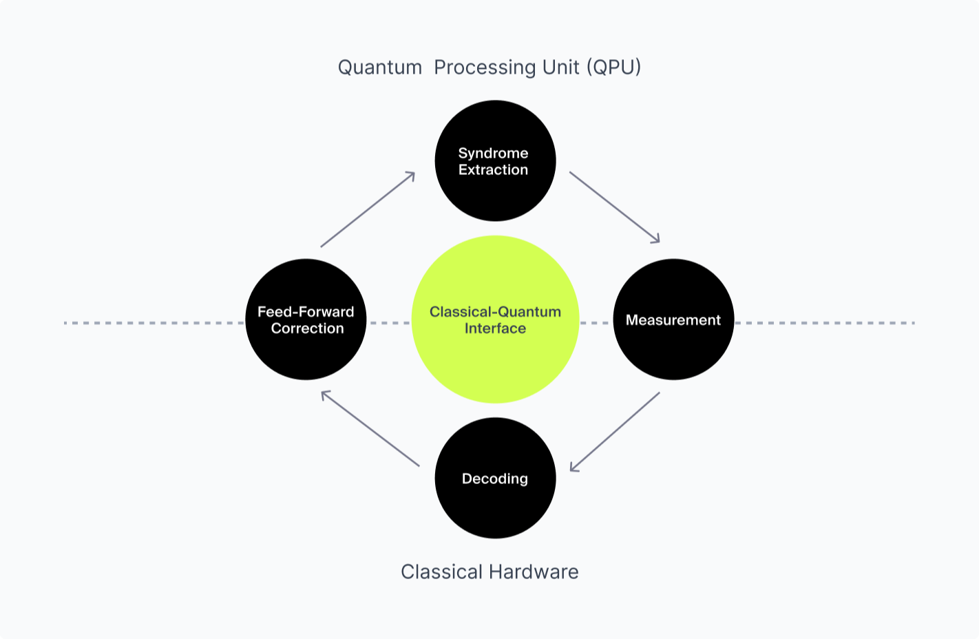
Layer 3: System Integration

The layers above describe individual components; the system integration layer ties them together to enable continuous operation at scale. This includes the decoder, a classical computer that must:

• Measure or detect the outputs of the error correction inside the quantum machine (error “syndromes”)
• Decode those outputs, and issue corrections (“feed-forward”) in real time.

Decoding, measurement, and feed-forward in particular is handled by classical hardware or at the quantum-classical interface. It is a continuous operation that must maintain pace with the quantum system or errors will outrun the correction cycle. Moreover, the system must maintain coherence and stability not for microseconds but for hours or days. Critically, the system integration layer is where scaling penalties emerge most clearly: effects that are manageable at small scale (crosstalk, thermal load, control complexity) can become prohibitive as the system grows.

Thus, a good control layer is:

• Efficient — accurately performs measurement, decoding, and feed-forward with the minimum classical hardware
• Reliable — doesn’t introduce additional error that must also be corrected
• Fast — ensures that the logical cycle time does not exceed the coherence constraint given by the physical layer

One "Trick" or Logical Cycle

Layer 4: Algorithm Demand

The top of the stack defines the bar the lower levels must reach in order to achieve a useful result. For a CRQC, the target is running Shor’s algorithm against cryptographic keys. This sets specific requirements: the number of logical qubits needed, the circuit depth, and the degree of parallelism the algorithm supports. Crucially, algorithmic optimizations lower the demand side of this equation: every improvement in how Shor’s algorithm is implemented reduces the requirements that the hardware stack must meet. This is why the resource estimates in the table below have fallen so dramatically: better algorithms are pulling the target closer from above while better hardware pushes capability upward from below.

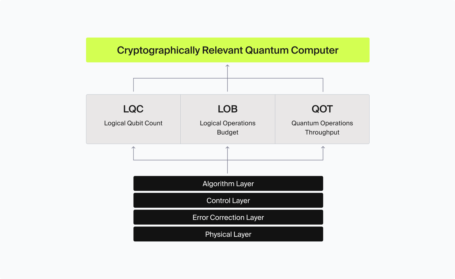
The algorithm choice and optimizations set the demand requirements, which must be matched with a sufficient “supply” of resources from the quantum computer, broken down into three composite metrics derived from a combination of factors across the quantum computing stack:

LQC — Logical Qubit Capacity

The number of error-corrected logical qubits available simultaneously — the quantum equivalent of how much working memory the system has; or, equivalently, the “width” of the quantum circuit.

LOB — Logical Operations Budget

The total number of reliable logical operations the system can execute before accumulated errors corrupt the computation; or, equivalently, the maximum “depth” of the quantum circuit.

QOT — Quantum Operations Throughput

The speed at which logical operations execute, measured in operations per second — analogous to “clockspeed” on a classical processor. Determines whether a theoretically possible algorithm runs in a human-scale practical timeframe. Also called CLOPS [8].

Cryptographically Relevant Quantum Computer

To put these metrics in context using Gidney 2025:

• Breaking RSA-2048 or ECDSA is estimated to require roughly 1,000 logical qubits (LQC = 1000). Today, the state of the art is a handful of logical qubits.
• The latest variants of Shor’s algorithm require on the order of a trillion logical gate operations (LOB = 10¹²). To date, no quantum computer has run more than a few thousand gate operations.
• A time target for RSA-2048 factoring is approximately one week. No quantum computer has yet demonstrated fault-tolerant logical operation at any meaningful duration required for such a computation, implying a QOT of one microsecond.

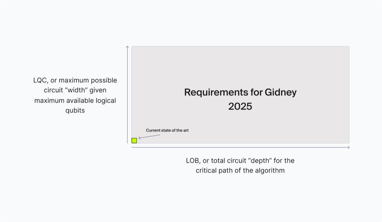
As Figure 10 shows, LQC and LOB have a geometric interpretation and can be combined into a single quantity sometimes called circuit “volume”:

Volume = LQC (width) × LOB (useable depth)

LCC = Volume × QOT

The choice of algorithm defines the threshold a quantum computer must reach. Variations of Shor’s algorithm often exploit a time-space tradeoff: faster runtimes require greater LQC and larger LOB, while slower runtimes expand LOB further.

Even with sufficient LCC, a quantum computer is only cryptographically relevant if it operates on a human timescale. QOT is therefore a practical constraint, not just an implementation detail.